본 게시물은 캐글 노트북을 바탕으로 작성되었습니다.
노트북을 보며 필사하면서 간단한 번역, 코드 리뷰를 작성했습니다.
이 노트북에서 우리는 bag of words와 tf-idf같은 문자 인코딩 기술이 어떻게 동작하는지 살펴보겠습니다. 이번 과제는 문자의 감성분석입니다. 우리가 사용할 데이터는 감성 정도(?)가 0,1,2,3,4로 라벨링 되어있는 영화 리뷰데이터 입니다. 0은 negative(부정), 1은 somehow negative(약간 부정), 2는 neutral(보통), 3은 somehow positive(약간 긍정), 4는 positive(긍정)으로 이루어져 있습니다.
먼저 EDA를 진행하고 머신러닝 모델링을 해보겠습니다.
필요한 라이브러리 불러오기
import pandas as pd
import numpy as np
import matplotlib.pyplot as plt
import seaborn as sns

from nltk.tokenize import word_tokenize
from nltk.corpus import stopwords
from nltk.probability import FreqDist
from nltk import ngrams
import string, re

from sklearn.feature_extraction.text import CountVectorizer, TfidfVectorizer
from sklearn.model_selection import train_test_split
from sklearn.linear_model import LogisticRegression
from sklearn.metrics import accuracy_score

import warnings, os
경고 문자를 무시해주고 matplotlib stylesheet 종류와 사이즈를 변경해줍니다
plt.figure(figsize=(16,7))
plt.style.use('ggplot')
warnings.filterwarnings('ignore')
먼저 데이터를 불러옵니다.
train = pd.read_csv('.../train.tsv.zip', sep='\t')
test = pd.read_csv('.../test.tsv.zip', sep='\t')
Part 1 탐색적 데이터 분석(EDA)
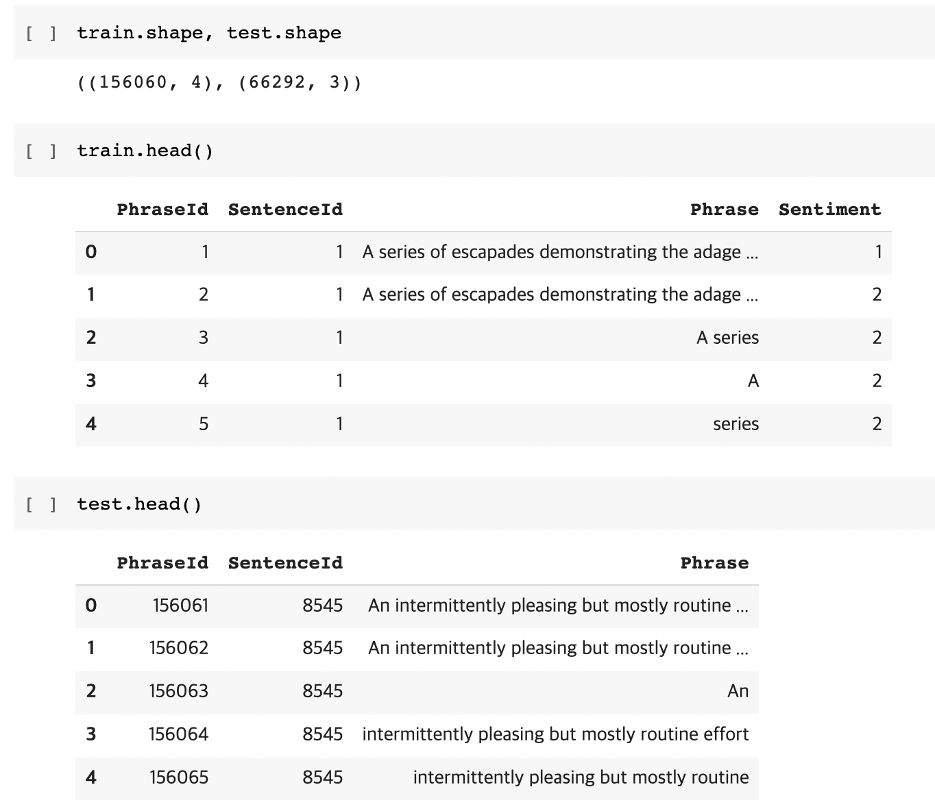
- 먼저 shape함수를 이용해 row, column개수를 확인 합니다.
- train.head(), tail.head()를 이용해 데이터가 어떤식으로 이루어졌는지 대략적으로 확인 합니다.
데이터들의 전체적인 자료형과 메모리 사용량 등을 확인하고, 결측치가 있는지 확인 해줍니다.

감성 설명
데이터의 sentiment 등급 마다 감정에 대한 설명을 추가해줍니다.
trian['sentiment_class'] = train['Sentiment'].map({0:'negative', 1:'somehow negative', 2:'neutral', 3:'somehow positive', 4:'positive'})
train.head()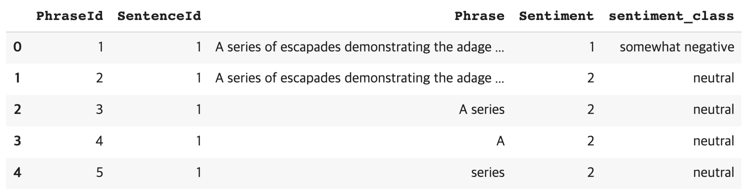
구두점 제거
def remove_punctuation(text):
  return ''.join([t for t in text if t not in string.punctuation])
train['Phrase'] = train['Phrase'].apply(lambda x : remove_punctuation(x))
train.head()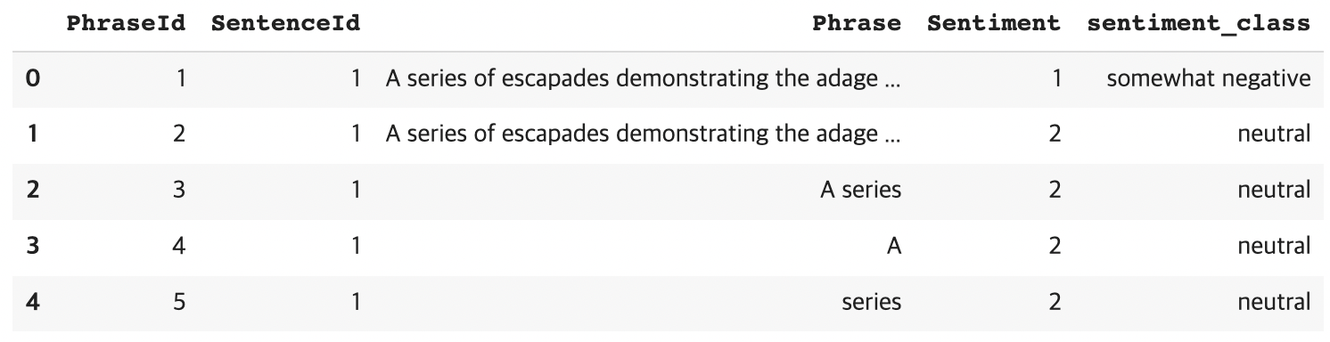
2개 이하의 문자로 이루어진 단어 제거
def words_with_more_than_three_chars(text):
  return ' '.join([t for t in text.split() if len(t) > 3])

train['Phrase'] = train['Phrase'].apply(lambda x : words_with_more_than_three_chars(x))
train.head()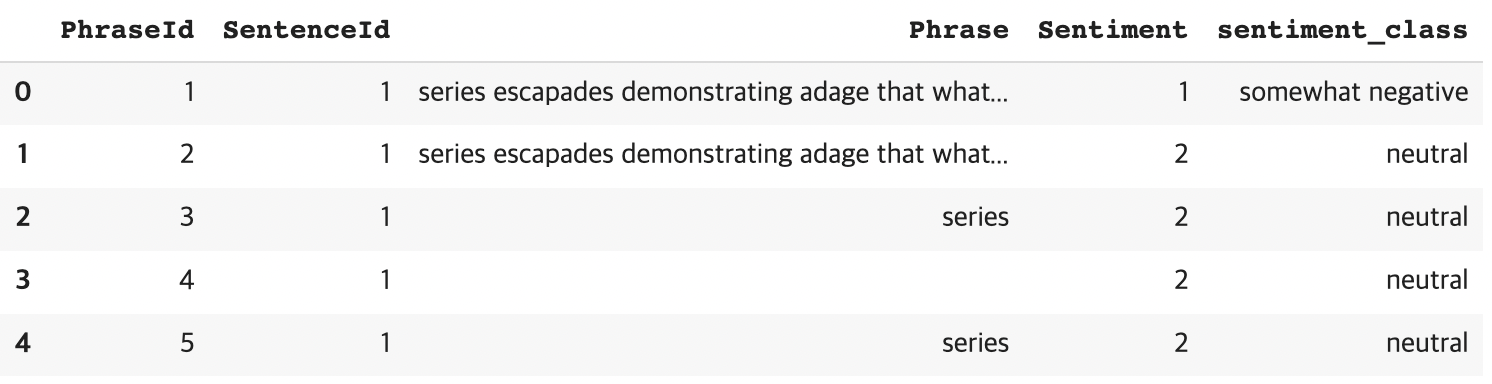
불용어 제거
nltk에 내장되어 있는 stopwords(불용어)를 다운로드 받아서 적용해줍니다.
import nltk
nltk.download('stopwords')

stop_words = stopwords.words('english')
train['Phrase'] = train['Phrase'].apply(lambda x : ' '.join([word for word in x.split() if word not in stop_words]))
train.head()
감성 카테고리 확인
train.groupby('Sentiment')['Sentiment'].count()타겟 클래스들 분포 시각화
train.groupby('sentiment_class')['sentiment_class'].count().plot(kind='bar', title='Target class', figsize=(16,7), grid=True)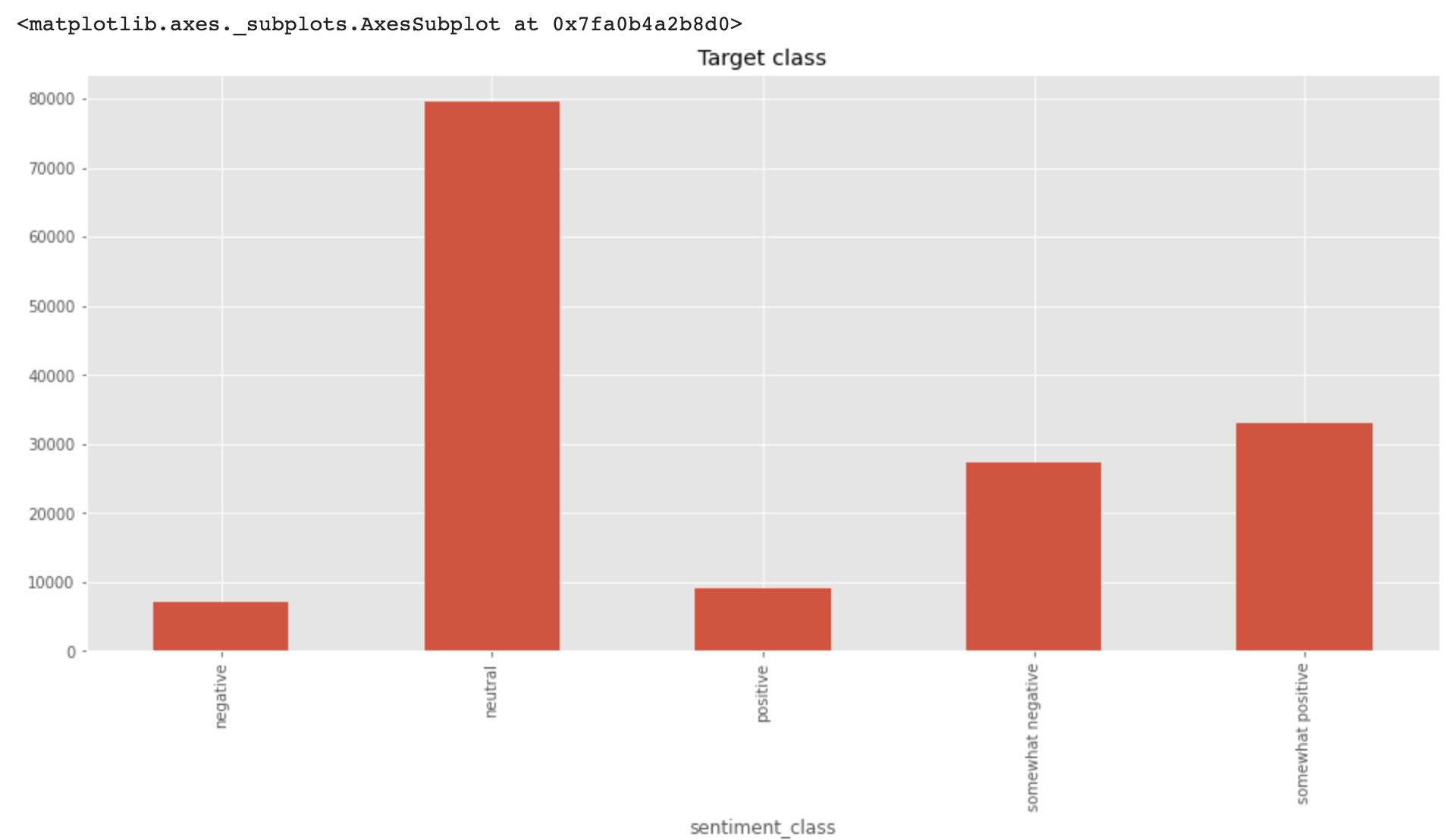
각 클래스들의 비율 시각화
((train.groupby('sentiment_class')['sentiment_class'].count() / train.shape[0])*100).plot(kind='pie', figsize=(7,7), title='% Target class', autopct='%1.0f%%')
문장의 길이 컬럼 추가
train['PhraseLength'] = train['Phrase'].apply(lambda x : len(x))
train.sort_values(by='PhraseLength', ascending=False).head()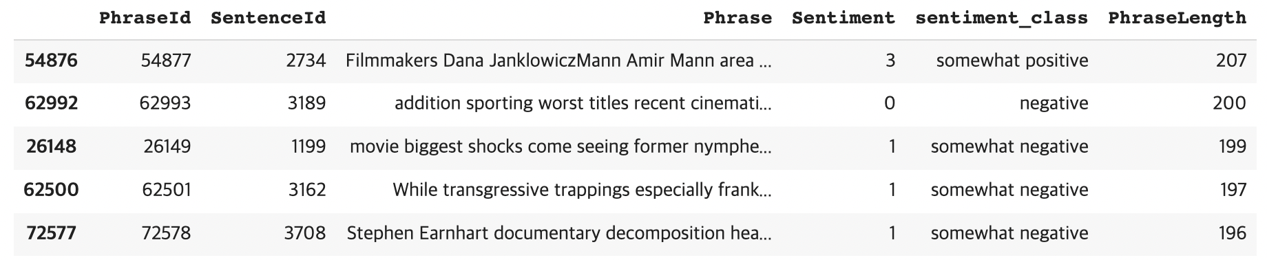
각 클래스에 대한 문장의 길이 분포 시각화
plt.figure(figsize=(16,7))
bins = np.linspace(0,200,50)
plt.hist(train[train['sentiment_class']=='negative']['PhraseLength'], bins=bins, density=True, label='negative')
plt.hist(train[train['sentiment_class']=='somehow negative']['PhraseLength'], bins=bins, density=True, label='somehow negative')
plt.hist(train[train['sentiment_class']=='neutral']['PhraseLength'], bins=bins, density=True, label='neutral')
plt.hist(train[train['sentiment_class']=='somehow positive']['PhraseLength'], bins=bins, density=True, label='somehow positive')
plt.hist(train[train['sentiment_class']=='positive']['PhraseLength'], bins=bins, density=True, label='positive')
plt.xlabel('Phrase length')
plt.legend()
plt.show()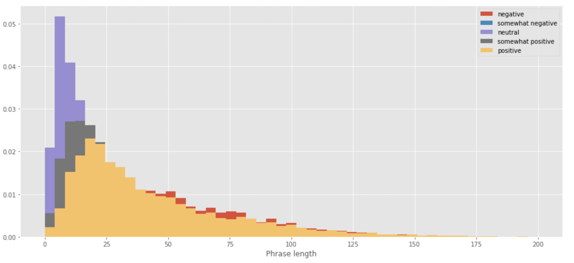
word cloud를 이용해 자주 나오는 단어 시각화
# Install wordcloud library
!pip install wordcloud

from wordcloud import WordCloud, STOPWORDS
stopwords = set(STOPWORDS)

word_cloud_common_words=[]
for index, row in train.itterrows():
  word_cloud_common_words.append((row['Phrase']))
 word_cloud_common_words

 wordcloud = WordCloud(width = 1600, height=800, backgroud_color = 'white', stopwords=stopwords,
                       min_font_size=5).generate(''.join(word_cloud_common_words))

# plot the WordCloud image
plt.figure(figsize=(16,8), facecolor=None)
plt.imshow(wordcloud)
plt.axis=('off')
plt.tight_layout(pad=0)

plt.show()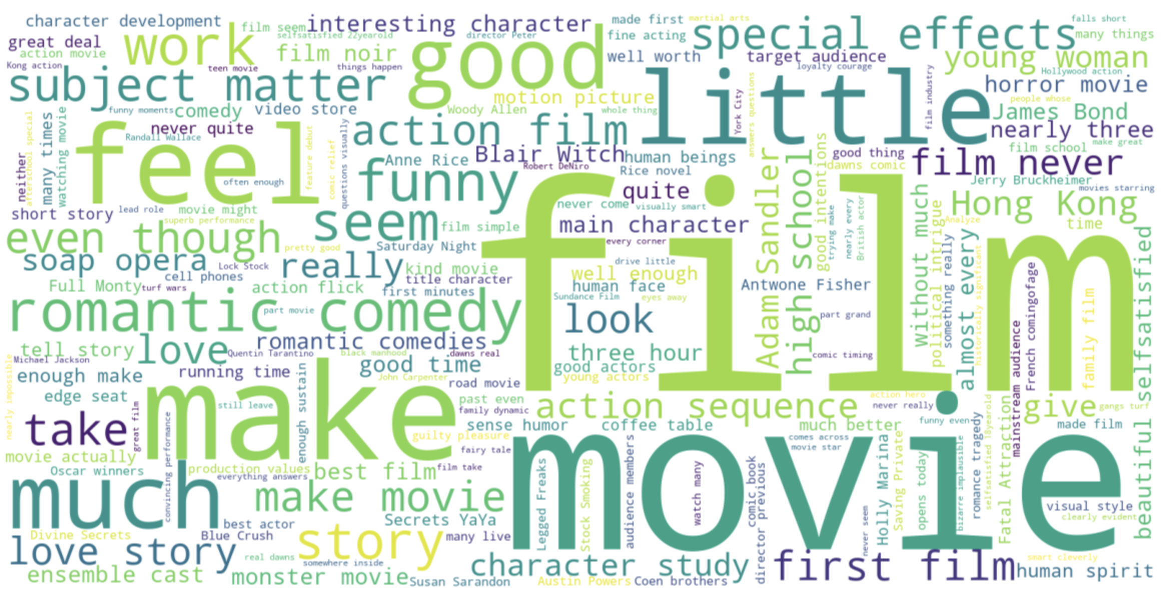
단어의 빈도수 체크
nltk.download('punkt')

text_list=[]
for index, row in train.iterrows():
  text_list.append((row['Phrase']))
 text_list

 total_words = ''.join(text_list)
 total_words=words_tokenize(total_words)

 freq_words = FreqDist(total_words)
 word_frequency=FreqDist(freq_words)

 # 10 common words
 print(word_frequency.most_common(10))
[('film', 3259), ('movie', 2892), ('like', 1968), ('story', 1204), ('much', 1085), ('good', 1069), ('even', 1041), ('characters', 994), ('little', 976), ('make', 838)]
pd.DataFrame(word_frequency, index=[0])
- 여기서 의문점 하나
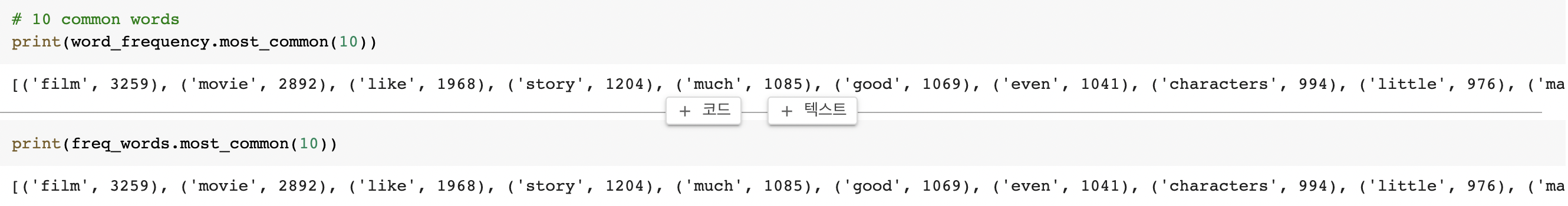
두 개의 결과가 같게 나오는데 왜 굳이 두 번의 FreqDist를 사용했는지 모르겠음...
# visualize
pd.DataFrame(word_frequency, index=[0]).T.sort_values(by=[0], ascending=False).head(20).plot(kind='bar', figsize=(16,6), grid=True)
부정적인 감성을 표현할 때 자주 사용된 단어
neg_text_list=[]
for index, row in train[train['Sentiment']=='negative'].iterrows():
  neg_text_list.append((row['Phrase']))
 neg_text_list

 neg_total_words = ' '.join(neg_text_list)
 neg_total_words = word_tokenize(neg_total_words)

 neg_freq_words=FreqDist(neg_total_words)
 neg_word_frequency=FreqDist(neg_freq_words)
여기도 굳이 같은 결과가 나오는데 FreqDist를 두 번 사용함

# visualize
pd.DataFrame(neg_word_frequency, index=[0].T.sort_values(by=[0], ascending=False).head(20).plot(kind='bar', figsize=(16,6), grid=True)
긍정적 감성에 자주 사용된 단어
pos_text_list=[]
for index, row in train[train['Sentiment']=='positive'].iterrows():
  pos_text_list.append((row['Phrase']))
 pos_text_list

 pos_total_words = ' '.join(pos_text_list)
 pos_total_words = word_tokenize(pos_total_words)

 pos_freq_words = FreqDist(pos_total_words)
 pos_word_frequency = FreqDist(pos_freq_words)

 #visualize
 pd.DataFrame(pos_word_frequency, index=[0]).T.sort_values(by=[0], ascending=False).head(20).plot(kind='bar', figsize=(16,6), grid=True)
긍정적인 감성 표현에 자주 사용되는 bigram 단어
n-gram = 단어마다 그 단어 포함 뒤로 n개만큼의 단어를 한 묶음으로 보고 이를 하나의 토큰으로 간주 하는 것.
- n = 1 : unigrams
- n = 2 : bigrams
- n = 3 : trigrams
- n >= 4 : ngrams
# n-gram 예시

text = 'Tom and Jerry love mickey. But mickey dont love Tom and Jerry. What a love mickey is getting from these two friends'
bigram_frequency = FreqDist(ngrams(word_tokenize(text), 3))
bigram_frequency.most_common()[0:5]
[(('Tom', 'and', 'Jerry'), 2),
(('and', 'Jerry', 'love'), 1),
(('Jerry', 'love', 'mickey'), 1),
(('love', 'mickey', '.'), 1),
(('mickey', '.', 'But'), 1)]
text_list = []
for index, row in train.iterrows():
text_list.append((row['Phrase']))
text_list
total_words = ' '.join(text_list)
total_words = word_tokenize(total_words)
freq_words = FreqDist(total_words)
word_frequency = FreqDist(ngrams(freq_words, 2))
word_frequency.most_common()[0:5]
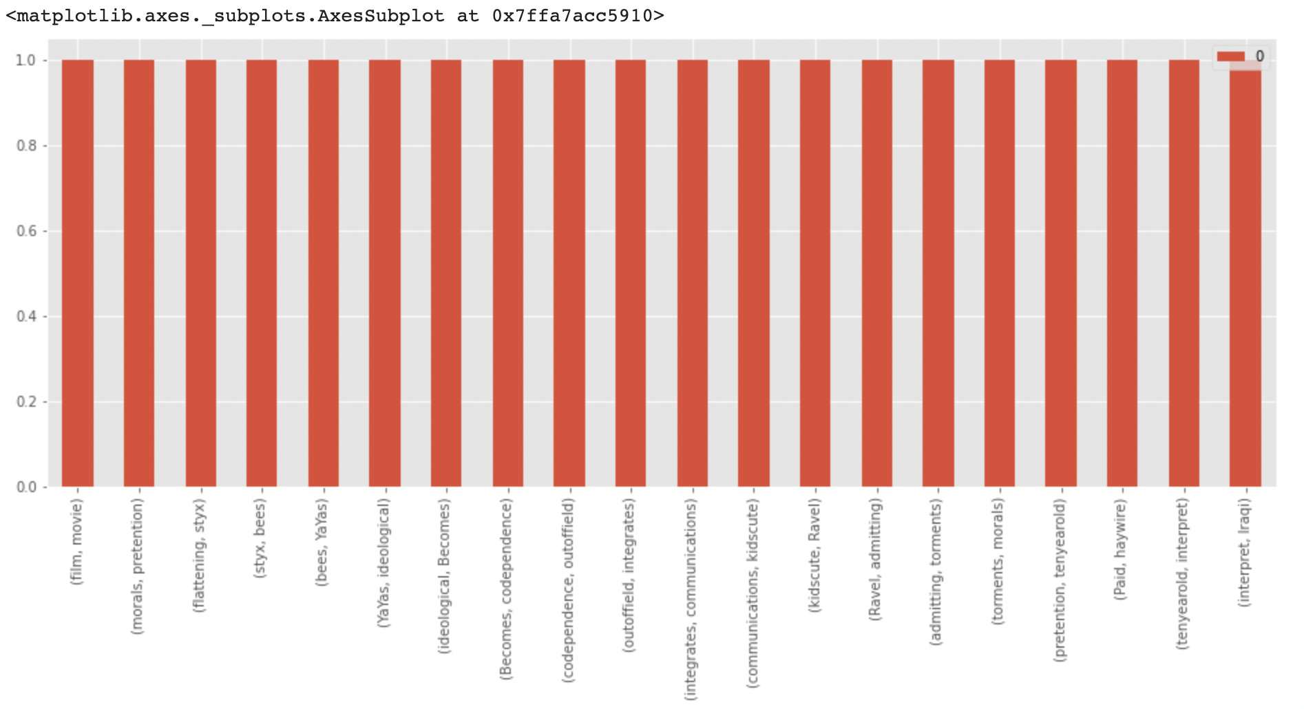
# visualize
pd.DataFrame(word_frequency, index=[0]).T.sort_values(by=[0], ascending=False).head(20).plot(figsize=(16,6), kind='bar', grid=True)
Part 2 Machine Learning Modeling
훈련 데이터 준비
CounterVectorizer를 이용해 Bag of words 생성
train['tokenized_words'] = train['Phrase'].apply(lambda x : word_tokenize(x))
train.head()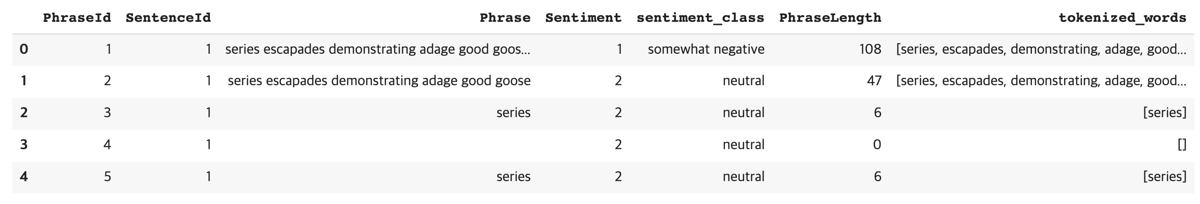
count_vectorizer = CountVectorizer()
phrase_dtm = count_vectorizer.fit_transform(train['Phrase']

phrase_dtm.shape
(156060, 15746)
훈련, 평가 데이터셋 비율 7:3으로 데이터 나눠줌
X_train, X_val, y_train, y_val = train_text_split(phrase_dtm, train['Sentiment'], text_size=0.3, random_state=38)
print(f'X_train shape : {X_train.shape}')
print(f'y_train shape : {y_train.shape}')
print(f'X_val shape : {X_val.shape}')
print(f'y_val shape : {y_val.shape}')
X_train shape : (109242, 15746)
y_train shape : (109242,)
X_val shape : (46818, 15746)
y_val shape : (46818,)
Logistic Regression 모델 훈련
model = LogisticRegression()
model.fit(X_train, y_train)

# 모델 평가

accuracy_score(model.predict(X_val), y_val) * 10063.75752915545303Tf-idf 를 이용해 모델 훈련
# tf-idf 사용을 위한 메모리 초기화
del X_train
del X_val
del y_train
del y_val

# tf-idf를 이용해 데이터 주닙
tfidf = TfidfVectorizer()
tfidf_dtm = tfidf.fit_transform(train['Phrase'])

X_train, X_val, y_train, y_val = train_test_split(tfidf_dtm, train['Sentiment'], test_size=0.3, random_state=38)
print(f'X_train shape : {X_train.shape}')
print(f'y_train shape : {y_train.shape}')
print(f'X_val shape : {X_val.shape}')
print(f'y_val shape : {y_val.shape}')
X_train shape : (109242, 15746)
y_train shape : (109242,)
X_val shape : (46818, 15746)
y_val shape : (46818,)tfidf_model = LogisticRegression()
tfidf_model.fit(X_train, y_train)
accuracy_score(tfidf_model.predict(X_val), y_val)*10062.37985390234525새로운 데이터 예측 함수
def predict_new_text(text):
  tfidf_text = tfidf.transform([text])
  return tfidf_model.predict(tfidf_text)

predict_new_text('The movie is bad ann sucks!')array([0])테스트 데이터 준비 & 예측
test['Phrase'] = test['Phrase'].apply(lambda x : remove_punctuation(x))
test['Phrase'] = test['Phrase'].apply(lambda x : words_with_more_than_three_chars(x))
test['Phrase'] = test['Phrase'].apply(lambda x : ' '.join([word for word in x.split() if x not in stop_words]))
test_dtm = tfidf.transform(test['Phrase'])

# Predict with test data
test['Sentiment'] = tfidf_model.predict(test_dtm)
test.set_index=test['PhraseId']
test.head()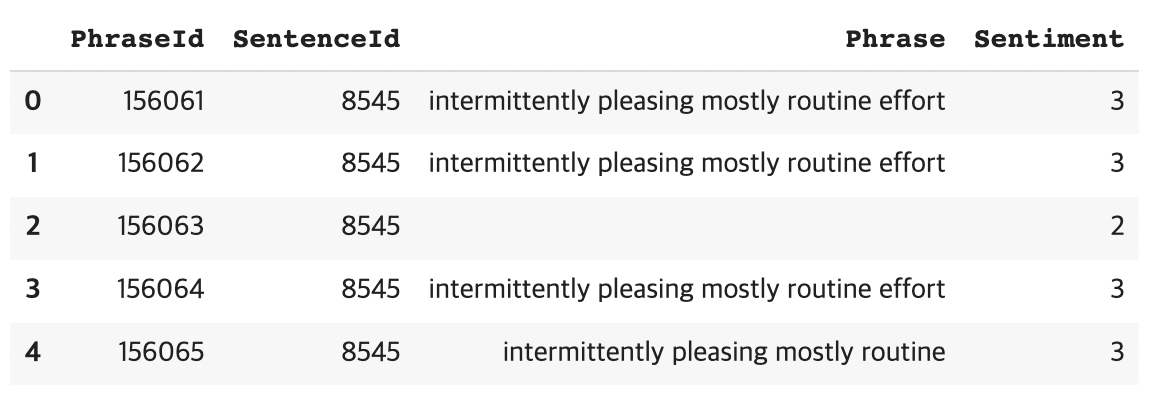
결과 csv 파일 저장
save results to csv file
test.to_csv('Submission.csv', columns=['PhraseId', 'Sentiment'], index=False)
'Kaggle 필사 & 리뷰 > NLP' 카테고리의 다른 글
| [NLP] Kaggle 필사 커리큘럼(진행중) (0) | 2022.10.04 |
|---|---|
| your first NLP competition submission (0) | 2022.09.18 |
| Getting started with NLP - A general Intro (0) | 2022.09.12 |

