본 게시물은 캐글 노트북을 바탕으로 작성되었습니다.
노트북을 보며 필사하면서 간단한 번역, 코드 리뷰를 작성했습니다.
Text classification step by step
자연어 처리(NLP)는 컴퓨터 과학, 인공 지능, 정보 공학, 그리고 인간-컴퓨터 상호작용 분야의 하위 분야입니다. 이 분야는 컴퓨터가 어떻게 엄청난 양의 자연어 데이터를 처리하고 분석하는지에 초점을 맞추고 있습니다. 언어를 이해하고 읽는 과정은 언뜻 보기에는 쉬워 보이지만 생각보다 더 복잡합니다.

목표
이번 커널의 목표는 다음과 같습니다.
- 기본적인 EDA
- 데이터 정제에 대한 기본 가이드
- 특징 분석과 추출
- 모델링과 평가지표
- 결과 제출
목차
Introduction
- 데이터 소개
Load and Check Data
- 라이브러리 불러오기
- 데이터셋 불러오기
EDA
- 타겟 레이블의 분포
- 트윗에 대한 분석
- 다른 레이블에 대한 분석
데이터 준비
- 데이터 정제
- 불용어 제거
- 토큰화
- 어간 추출
- 표제어 추출
- 데이터 나누기
특징 추출
- Bag of words
- Tf-idf Vectorizer
- Reduce the dimensionality of the Matrix
모델 훈련
- MultinomialNB
Introduction
About Data
- 어떤 파일이 필요한가요?
- train.csv, test.csv, sample_submission.csv - 학습 데이터와 시험 데이터는 다음과 같은 정보를 담고 있습니다.
- 트윗 내용
- 트윗 내용의 키워드
- 트윗을 보낸 위치 - 무엇을 예측하나요?
- 트윗이 실제 재난과 관련 있는지에 대한 여부(관련 있으면 1, 없으면 0)
데이터셋 칼럼들
- id : 각 트윗의 id
- text : 트윗의 내용
- location : 트윗을 보낸 위치
- keyword : 트윗 내용의 키워드
- target : 훈련 데이터에만 있는 칼럼으로 트윗이 실제 재난과 관련 있는지에 대한 값
Load and Check Data
필요한 모듈 불러오기
!pip install scikit-plotimport numpy as np
import pandas as pd
import re
import matplotlib.pyplot as plt
import seaborn as sns
import nltk
from sklearn import feature_extraction, model_selection, naive_bayes, pipeline, manifold, preprocessing
import nltk.corpus
from nltk.corpus import stopwords
from nltk.tokenize import BlanklineTokenizer
from nltk.tokenize import TweetTokenizer
nltk.download('punkt')
nltk.download('stopwords')
nltk.download('wordnet')
from nltk.stem import WordNetLemmatizer
import string
from nltk.util import ngrams
from sklearn.feature_extraction.text imoprt CountVectorizer
from collections import defaultdict, Counter
plt.style.use('ggplot')
stop=set(stopwords.words('english'))
import scikitplot as skplt
from nltk.tokenize import word_tokenize
import gensim
from keras.preprocessing.text import Tokenizer
from keras.preprocessing.sequence import pad_sequences
from tqdm import tqdm
from keras.models import Sequential
from keras.layers import Embedding, LSTM, Dense, SpatialDropout1D
from keras.initializers import Constant
from sklearn.model_selection import train_test_split
from tensorflow.keras.optimizers import Adam
from nltk.stem import PorterStemmer
from wordcloud import WordCloud
from sklearn.feature_extraction.text import TfidfVectorizer
import pickle
from multiprocessing import PoolImport Dataset
train_data = pd.read_csv('.../train.csv')
test_data = pd.read_csv('.../test.csv')

train_data.head(10)print('There are {} rows and {} columns in train'.format(train_data.shape[0], train_data.shape[1]))
print('There are {} rows and {} columns in test'.format(test_data.shape[0], test_data.shape[1]))
# outputs
There are 7613 rows and 5 columns in train
There are 3263 rows and 4 columns in testtrain_data.dtypes
# 데이터의 유형 확인
id int64
keyword object
location object
text object
target int64
dtype: objectEDA
타깃 레이블의 분포
시작 전에 먼저 타깃 레이블의 분포를 확인 해봅시다. 타겟 레이블의 값은 단 두 개의 클래스 0, 1로 구성되어 있습니다.
x = train_data.target.value_counts()
sns.barplot(x.index, x)
plt.gca().set_ylabel('samples')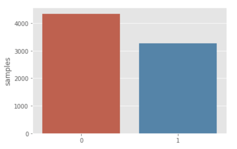
클래스 0(재난과 관련 없는)인 트윗이 클래스 1(재난과 관련 있는)인 트윗보다 많습니다.
트윗 분석
먼저, 우리는 아주 기본적인 분석을 진행해보겠습니다. 문자 수준, 단어 수준, 문장 수준 분석이 바로 그것입니다.
트윗에 있는 문자의 수
fig, (ax1, ax2) = plt.subplots(1, 2, figsize=(10,5))
tweet_len = train_data[train_data['target']==1]['text'].str.len() # 학습 데이터에서 타겟 클래스의 값이 1인 인덱스 중에서 'text'에 있는 문자의 길이
ax1.hist(tweet_len, color='blue')
ax1.set_title('disaster_tweets')
tweet_len = train_data[train_data['target']==0]['text'].str.len()
ax2.hist(tweet_len, color='CRIMSON')
ax2.set_title('Not disaster tweets')
fig.suptitle('Characters in tweets')
plt.show()
두 개의 분포가 거의 비슷합니다. 120에서 140개의 문자가 있는 트윗이 두 개 모두에서 가장 많습니다.
트윗에 있는 단어의 수
fig, (ax1, ax2) = plt.subplots(1, 2, figsize=(10,5))
# 학습 데이터의 타겟 클래스가 1인 인덱스들의 'text'에 몇 개의 단어가 있는지 확인
# 판다스에서 문자열 관련 함수를 사용하거나 전처리를 할 때 함수 앞에 str 붙여줘야함
tweet_len = train_data[train_data['target']=1]['text'].str.split().map(lambda x : len(x))
ax1.hist(tweet_len, color='blue')
ax1.set_title('disaster tweets')
tweet_len = train_data[train_data['target']==0]['text'].str.split().map(lambda x : len(x))
ax2.hist(tweet__len, color='CRIMSON')
ax2.set_title('disaster tweets')
fig.suptitle('Words in a tweet')
plt.show()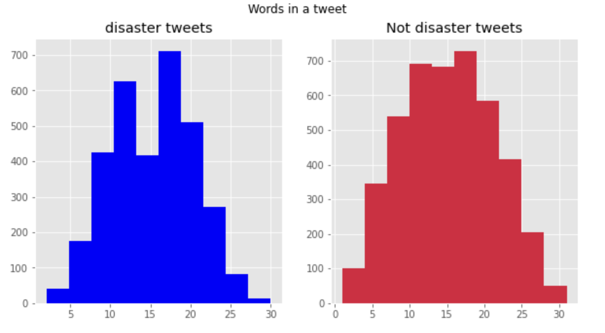
트윗에 있는 단어 길이의 평균
fit, (ax1, ax2) = plt.subplots(1, 2, figsize=(10,5))
word = train_data[train_data['target']==1]['text'].str.split().apply(lambda x : [len(i) for i in x])
sns.distplot(word.map(lambda x : np.mean(x)), ax=ax1, color='red')
ax1.set_title('disaster')
word = train_data[train_data['target']==0]['text'].str.split().apply(lambda x : [len(i) for i in x])
sns.distplot(word.map(lambda x : np.mean(x)), ax=ax1, color='green')
ax2.set_title('Not disaster')
fig.suptitle('Average word length in each tweet')
plt.show()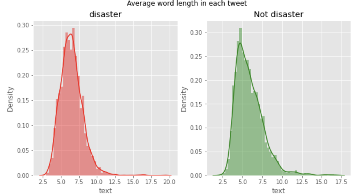
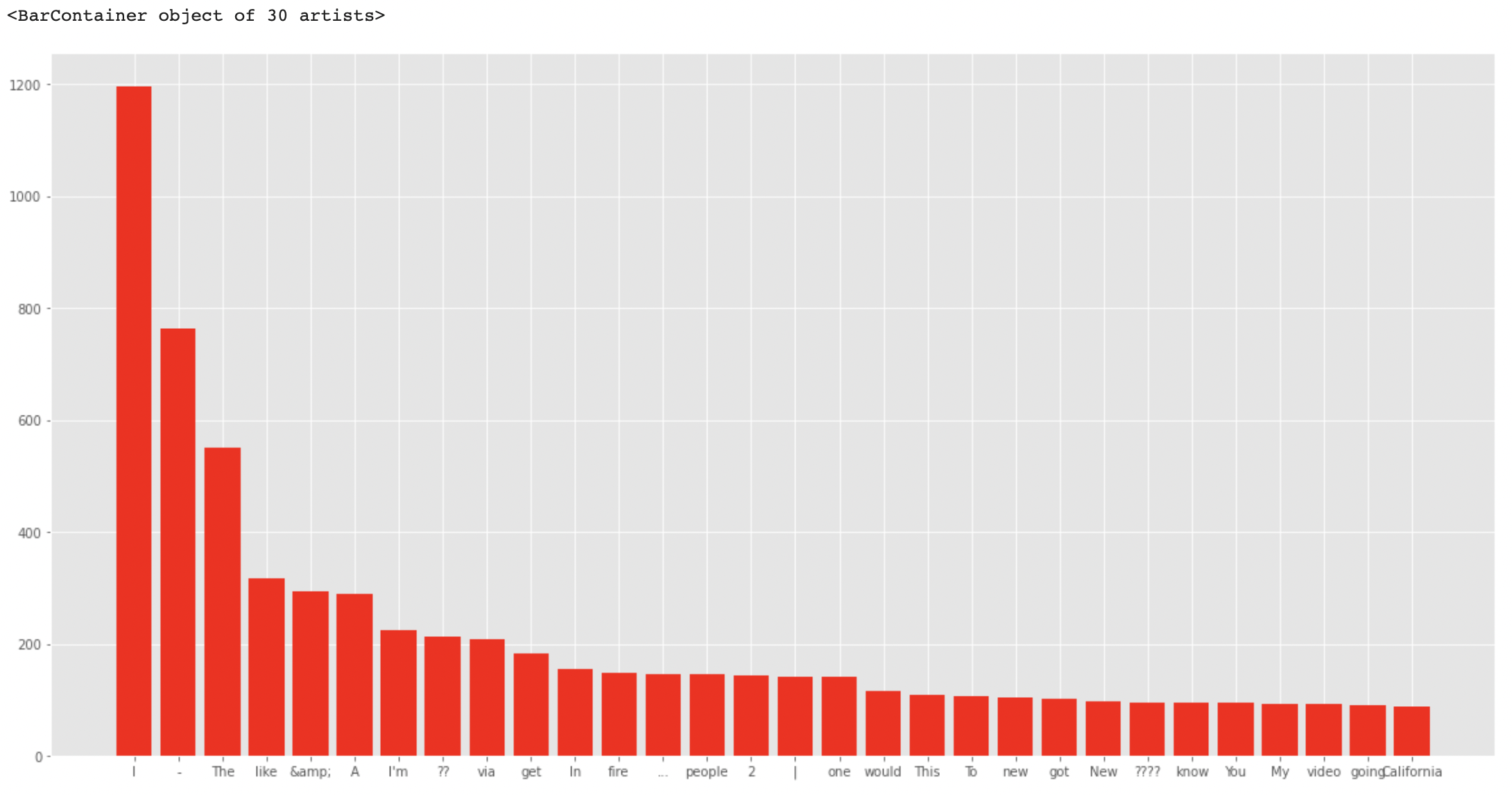
이번에는 말뭉치 전체에서 각 단어들의 빈도를 보겠습니다.
corpus = []

for x in train_data['text'].str.split():
  for i in x:
    corpus.append(i)

dic = defaultdict(int)
for word in corpus:
  # 단어가 불용어가 아니라면 딕셔너리에 추가
  if word not in stop:
    dic[word] += 1

top = sorted(dic.items(), key=lambda x : x[1], reverse=True)[:30] # 1

x, y = zip(*top) # 2
plt.rcParams['figure.figsize'] = (20, 10)
plt.bar(x, y, color='red')
# 1
- dic.items() : [ (key 1, value 1), (key 2, value 2), ...] 형식의 리스트 반환
- key = lambda x : x[1] : 리스트에서 하나씩 꺼낸다음(튜플) 인덱스 1(value) 기준으로 정렬
- reverse=True : 내림차순 정렬
# 2
- 애스터리스크(*) : 현재 리스트인 top을 unpacking해줌
from nltk.corpus imoprt stopwords
stop = stopwords.words('english')
dic = defualtdict(int)
for word in corpus:
  # 단어가 불용어라면 딕셔너리에 추가
  if word in stop:
    dic[word] += 1

top = sorted(dic.items(), key=lambda x : x[1], reverse=True)[:30]

x, y =zip(*top)
plt.rcParams['figure.figsize'] = (20, 10)
plt.bar(x, y, color='green')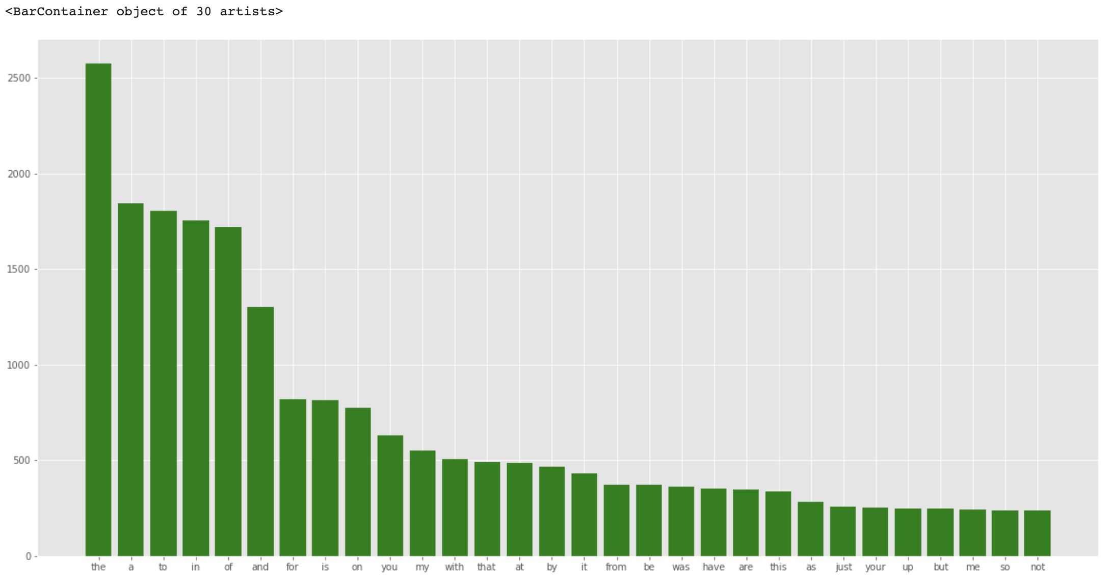
전체 트윗에서 구두점을 한 번 살펴보겠습니다.
plt.figure(figsize=(10,5))
import string
dic=defaultdict(int)
special = string.punctuation
for i in corpus:
  if i in special:
    dic[i] += 1

x, y = zip(*dic.items())
plt.barh(x, y, color = 'purple')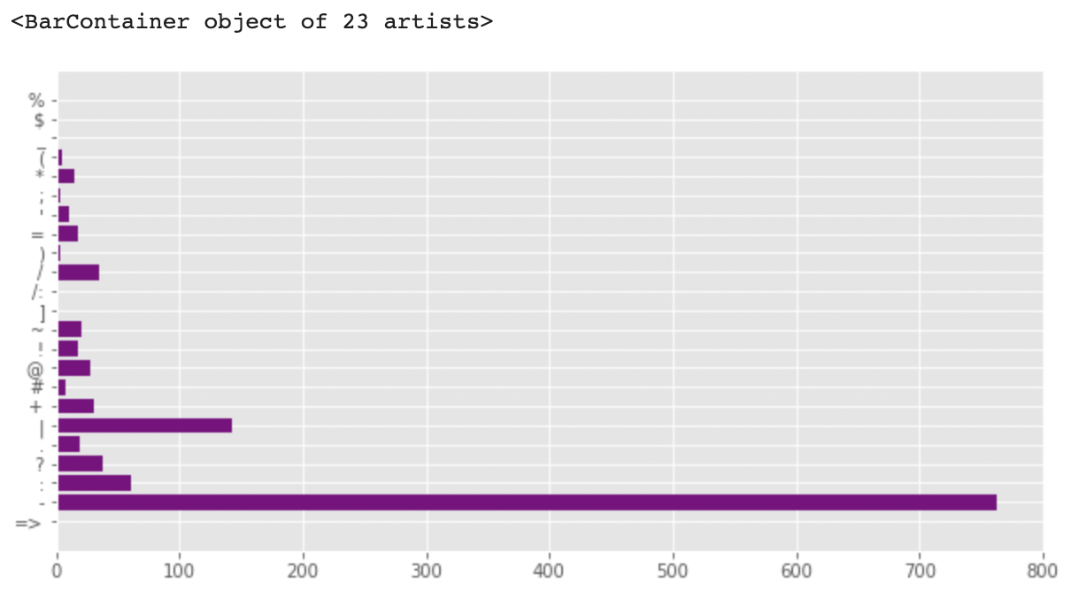
각 타깃 클래스에 대해서 좀 더 자세히 살펴보겠습니다.
# 타겟 클래스가 0인 텍스트에서 가장 빈도수가 높은 단어 상위 50개 출력
words = train_data[train_data.target==0].text.apply(lambds x : [word.lower() for word in x.split()])
h_words = Counter()

for text_ in words:
  h_words.update(text_) # h_words 갱신

print(h_words.most_common(50))
# 타겟 클래스가 1인 텍스트에서 빈도수가 가장 많은 단어 상위 50개 출력
words = train_data[train_data.target==1].text.apply(lambda x : [word.lower() for word in x.split()])
h_words = Counter()

for text_ in words:
  h_words.update(text_)

print(h_words.most_common(50))
다른 변수들에 대한 분석
keyword and location
1. 결측치
훈련 데이터와 테스트 데이터 모두 keyword와 location에서 동일한 결측치 비율을 가지고 있습니다.
0.8% 의 keyword가 훈련, 테스트 데이터에서 결측치이고, 33%의 location이 훈련, 테스트 데이터에서 결측치입니다. 두 데이터가 결측치 비율이 거의 동일한 걸로 봐서 아마 같은 샘플에서 가져온 것 같습니다. 해당 피쳐들에서의 결측치는 각각 no_keyword와 no_location으로 채워집니다.
missing_cols = ['keyword', 'location']

fig, axes = plt.subplots(ncols = 2, figsize = (17,4), dpi=100) # dpi : dot per inch(default 100)

sns.barplot(x=train_data[missing_cols].isnull().sum().index, y=train_data[missing_cols].isnull().sum().values, ax=axes[0])
sns.barplot(x=test_data[missing_cols].isnull().sum().index, y=train_data[missing_cols].isnull().sum().values, ax=axes[1])

axes[0].set_ylabel('Missing Value Count', size=15, labelpad=20)
# tick_params 로 틱과 관련된 설정을 원하는대로 바꿔줌
axes[0].tick_params(axis='x', labelsize=15)
axes[0].tick_params(axis='y', labelsize=15)
# 두 개를 같은 사이즈로 바꾸는데 굳이 두번을?
# tick_params(axis='both', labelsize=15)로 하면 될것을..

axes[1].tick_params(axis='x', labelsize=15)
axes[1].tick_params(axis='y', labelsize=15)

axes[0].set_title('Training Set', fontsize=13)
axes[1].set_title('Test Set', fontsize=13)

plt.show()
1. 중복도와 타깃 분포
중복도란 전체 행에 대하여 특정 칼럼의 중복 수치를 나타내는 지표입니다. 만약 특정 칼럼이 전체 행에 대하여 중복되는 값이 많으면 중복도(Cardinality)가 낮다라고 합니다. 중복되는 값이 적으면 중복도(Cardinality)가 높다라고 합니다.
- 카디널리티가 높다 = 중복되는 값이 적다 = 유니크한 값이 많다
- 카디널리티가 낮다 = 중복되는 값이 많다 = 유니크한 값이 적다
location은 자동적으로 만들어지는 값이 아니라 유저가 입력하는 값입니다. 때문에 location 정보는 아주 지저분하고 유니크한 값이 많습니다. 이 칼럼은 피쳐로 쓸 수가 없습니다.
다행히도, 키워드의 단어들 중 일부는 오직 한 문맥에서만 사용될 수 있기 때문에 키워드에는 의미가 있습니다. 키워드는 트윗 수와 타깃이 의미하는 바와 큰 차이가 있습니다. 키워드는 그 자체로 특징으로 사용하거나 텍스트에 추가된 단어로 사용할 수 있습니다. 훈련 세트의 모든 키워드가 테스트 세트에 있습니다. 훈련과 테스트 세트가 동일한 샘플에서 온 경우 키워드에 타겟 인코딩을 사용할 수도 있습니다.
print(f'Number of unique values in keyword = {train_data['keyword'].nunique()} (Training) - {test_data['keyword'].nunique()} (test)')
print(f'Number of unique values in location = {train_data["location"].nunique()} (Training) - {test_data["location"].nunique()} (Test)')

#-----------------------------------------------------------------
# outputs
Number of unique values in keyword = 221 (Training) - 221 (test)
Number of unique values in location = 3341 (Training) - 1602 (Test)

#-----------------------------------------------------------------
train_data['target_mean'] = train_data.groupby('keyword')['target'].transform('mean')

fig = plt.figure(figsize=(8,72), dpi=100)

sns.countplot(y=train_data.sort_values(by='target_mean', ascending=False)['keyword'],
              hue=train_data.sort_values(by='target_mean', ascending=False)['target'])

plt.tick_params(axis='x', labelsize=15)
plt.tick_params(axis='y', labelsize=12)
plt.legend(loc=1)
plt.title('Target Distribution in Keywords')

plt.show()

train_data.drop(columns=['target_mean'], inplace=True)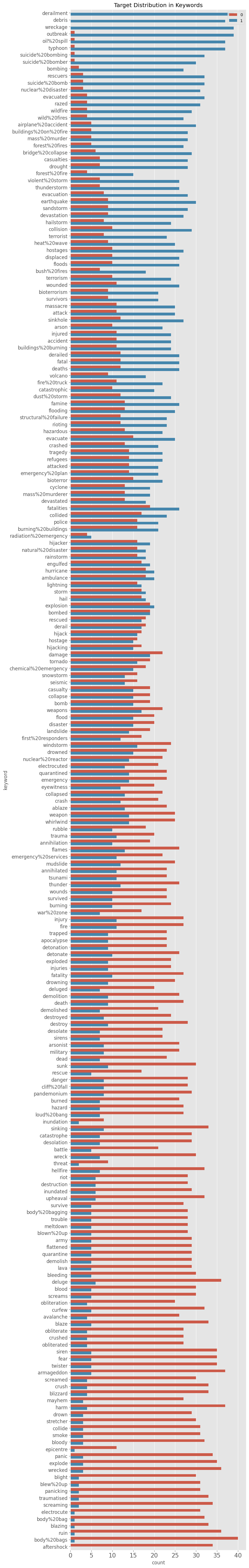
Hashtag 분석
# 로 태그 되어 있는 정보가 우리가 진행할 과제에 영향력이 있는지를 보기 위해 간단하게 해시태그 분석을 진행해보겠습니다.
정규 표현식
해시태그를 분석한다는 말은 해시태그부터 4자리의 문자를 살펴본다는 의미이고, 이 정도면 우리가 진행하는 문제에 있어서는 충분해 보입니다. 위 문자열은 원시 문자열(더 이상 백슬래쉬가 이스케이프 문자가 아님을 의미)로 정규식이 포함된 표준 관행입니다. regex = r'^(\d {4})'
def clean_text(df, text_field, new_text_field_name):
  df[new_text_field_name] = df[text_field].str.lower() # Convert strings in the Series/Index to lowercase

  # remove numbers
  df[new_text_field_name] = df[new_text_field_name].apply(lambda elem : re.sub(r"\d+", "", elem))
  # remove url
  df[new_text_field_name] = df[new_text_field_name].apply(lambda elem: re.sub(r"https?://\S+", "", elem))
  # remove HTML tags
  df[new_text_field_name] = df[new_text_field_name].apply(lambda elem : re.sub(r"<.*?>", "", elem))
  # remove emojis
  df[new_text_field_name] = df[new_text_field_name].apply(lambda elem: re.sub(r"["
                           u"\U0001F600-\U0001F64F"  # emoticons
                           u"\U0001F300-\U0001F5FF"  # symbols & pictographs
                           u"\U0001F680-\U0001F6FF"  # transport & map symbols
                           u"\U0001F1E0-\U0001F1FF"  # flags (iOS)
                           u"\U00002702-\U000027B0"
                           u"\U000024C2-\U0001F251"
                           "]+", "", elem))
  return df

data_clean = clean_text(train_data, 'text', 'text_clean')
data_clean_test = clean_text(test_data, 'text', 'text_clean')
data_clean.head()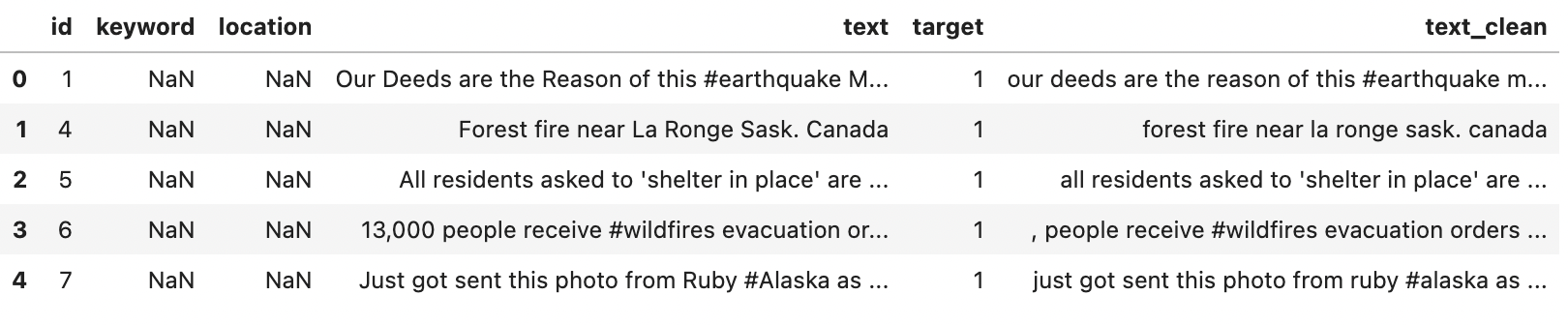
불용어 제거
from nltk.corpus import stopwords
stop = stopwords.words('english')
data_clean['text_clean'] = data_clean['text_clean'].apply(lambda x : ' '.join([word for word in x.split() if word not in stop]))
data_clean.head()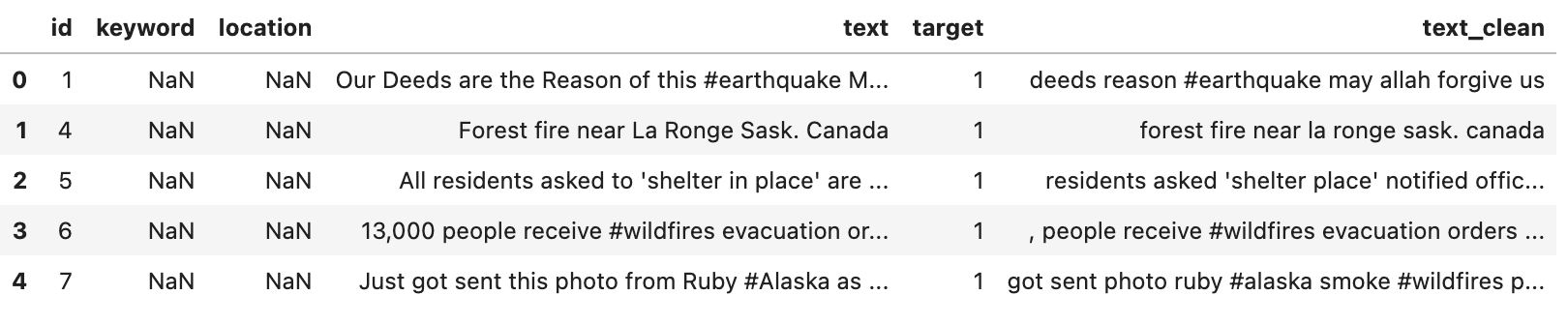
토큰화
from nltk.tokenize import sent_tokenize, word_tokenize
data_clean['text_tokens'] = data_clean['text_clean'].apply(lambda x : word_tokenize(x))
data_clean.head()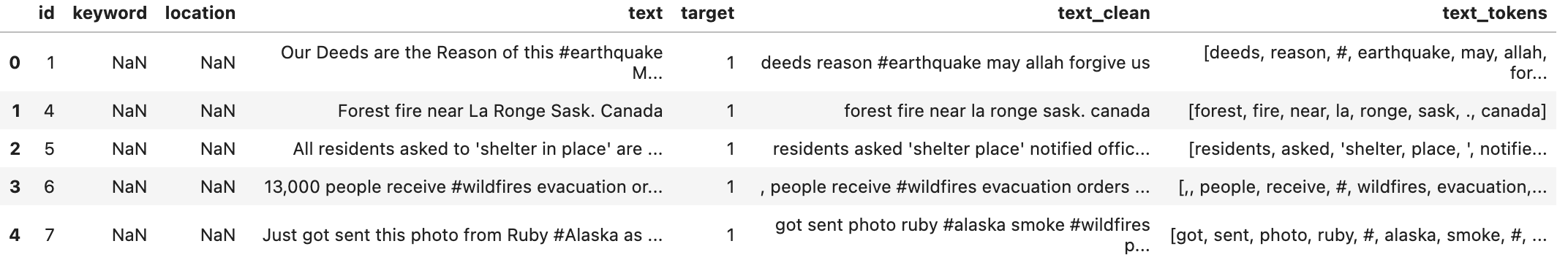
어간 추출
# Stemming
import nltk
from nltk.stem.porter import PorterStemmer
porter_stemmer = PorterStemmer()
text = 'studies studying cries cry'
tokenization = nltk.word_tokenize(text)
for w in tokenization:
  print('Stemming for {} if {}'.format(w, porter_stemmer.stem(w)))
# Lemmatization(표제어 추출)
from nltk.stem import WordNetLemmatizer
nltk.download('omw-1.4')

wordnet_lemmatizer = WordNetLemmatizer()
text = 'studies studying cries cry'
tokenization = nltk.word_tokenize(text)
for w in tokenization:
  print("Lemma for {} is {}".format(w, wordnet_lemmatizer.lemmatize(w)))
# 어떻게 진행되는지 살펴 봤으니 함수로 구현
def word_stemmer(text):
  stem_text = [PorterStemmer().stem(i) for i in text]
  return stem_text

data_clean['text_clean_tokens'] = data_clean['text_tokens'].apply(lambda x : word_stemmer(x))
data_clean.head()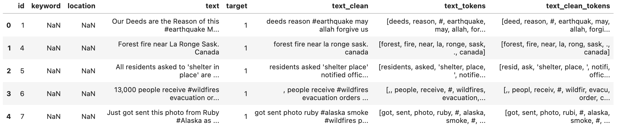
def word_lemmatizer(text):
  lem_text = [WordNetLemmatizer().lemmatize(i) for i in text]
  return lem_text

data_clean['text_clean_tokens'] = data_clean['text_tokens'].apply(lambda x : word_lemmatizer(x))
data_clean.head()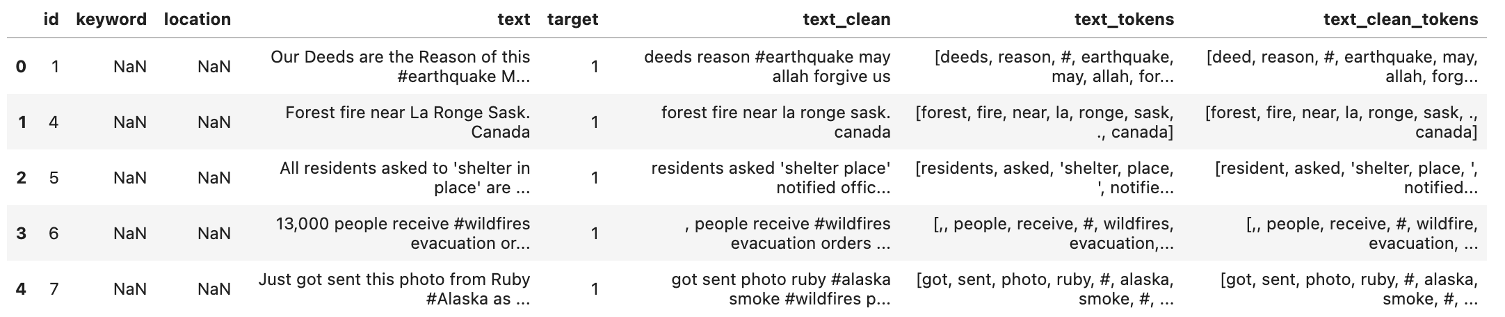
데이터 나누기
x_train, x_text, y_train, y_text = train_test_split(data_clean['text_clean'], data_clean['target'], test_size=0.2, random_state=10)

print(x_train.shape)
print(y_train.shape)
print(x_test.shape)
print(y_test.shape)
특징 추출 : tf-idf
Bag of words
벡터화는 텍스트 문서들의 모음을 숫자로 표현된 특징 벡터로 바꿔주는 일반적인 방법입니다. 토큰화, 카운팅, 정규화를 진행하는 특정한 방법은 bag of words 혹은, bag of n-grams라고 불립니다. 이러한 과정을 거치면 텍스트 문서는 단어들의 위치적인 특성은 고려하지 않은 채로 몇 번 등장하는지로만 설명됩니다.
CountVectorizer
CountVectorizer는 텍스트 문서를 토큰 단위의 행렬로 바꿔줍니다. 이 행렬은 문서에서 토큰이 얼마나 등장하는지에 대한 행렬입니다. 이렇게 만들어진 행렬은 횟수에 대한 희소 표현(?)을 해줍니다.
vectorizer = CountVectorizer(analyzer = 'word', ngram_range=(1,1))
vectorized = vectorizer.fit_transform(x_train)
pd.DataFrame(vectorized.toarray(), index=['sentence '+str(i) for i in range(1, 1+len(x_train))], columns=vectorizer.get_feature_names_out)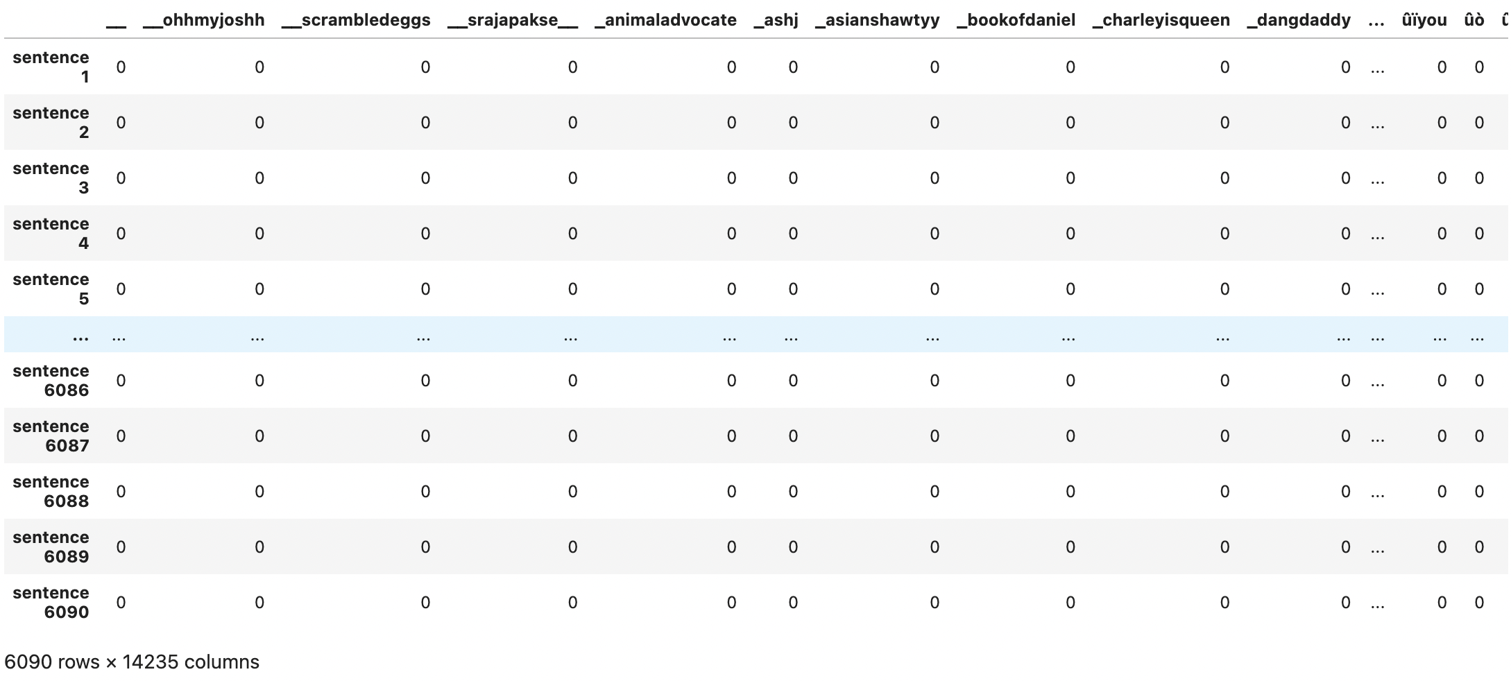
결과를 보면 토큰의 위치적인 정보가 전부 사라진 것을 볼 수 있습니다.
이번에 우리는 최소 3알 파벳 이상 있는 토큰만으로 만들어 보겠습니다.
# Only alphabet, contains at least 3 letters
vectorizer = CountVectorizer(analyzer='word', token_pattern=r'\b[a-zA-Z]{3,}\b', ngram_range=(1,1))
vectorized = vectorizer.fit_transform(x_train)
pd.DataFrame(vectorized.toarray(), index=['sentence '+str(i) for i in range(1, 1+len(x_train))], columns=vectorizer.get_feature_names_out())
vectorizer = CountVectorizer(analyzer='word', token_pattern=r'\b[a-zA-Z]{3,}\b', ngram_range=(2,2))

# only bigrams
vectorized = vectorizer.fit_transform(x_train)
pd.DataFrame(vectorized.toarray(), index=['sentence '+str(i) for i in range(1, 1+len(x_train))], columns=vectorizer.get_feature_names_out())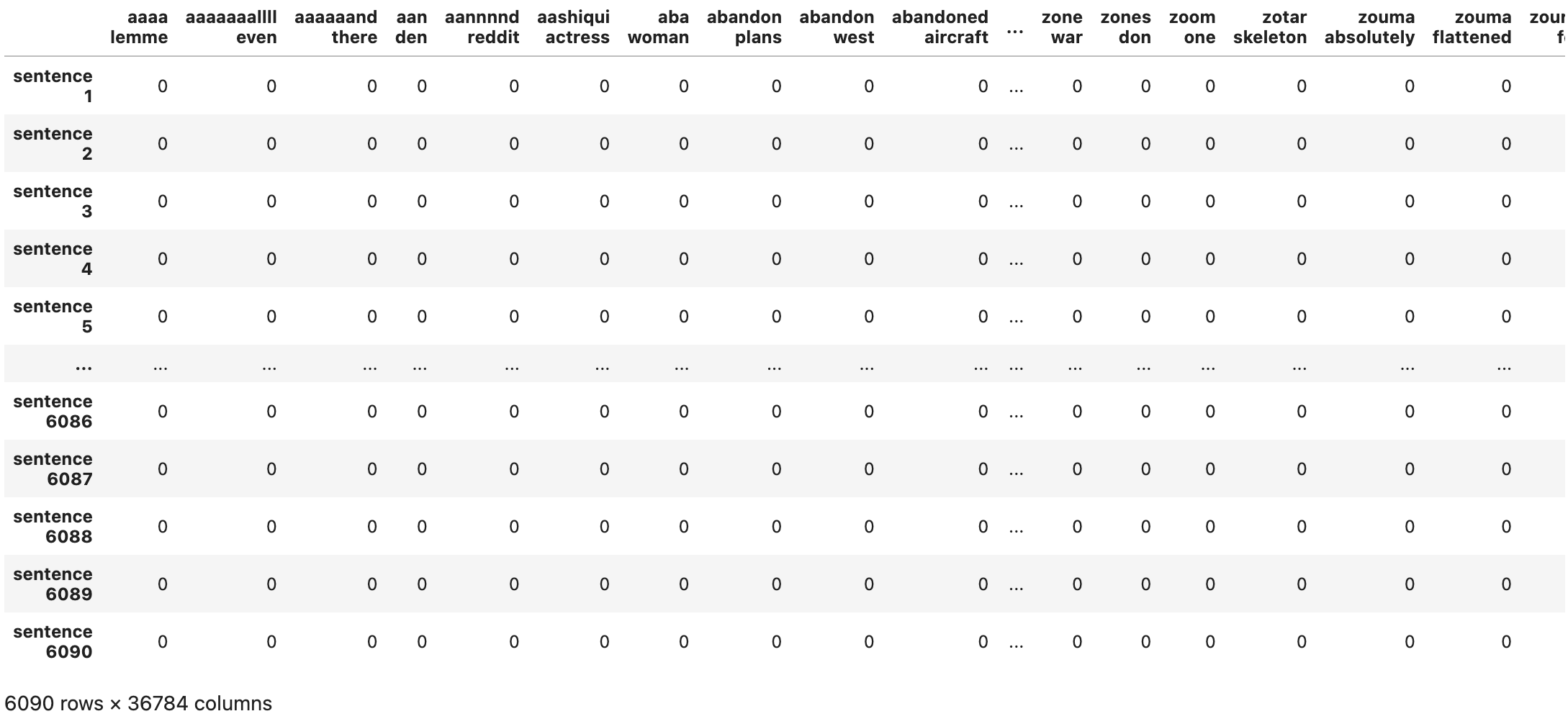
# consider both unigrams and bigrams, occur at least twice
vectorizer = CountVectorizer(analyzer = 'word', token_pattern=r'\b[a-zA-Z]{3,}\b', ngram_range=(1,2), min_df=2)
vectorized = vectorizer.fit_transfoem(x_train)
pd.DataFrame(vectorized.toarray(), index=['sentence '+str(i) for i in range(1, 1+len(x_train))], columns=vectorizer.get_feature_names_out())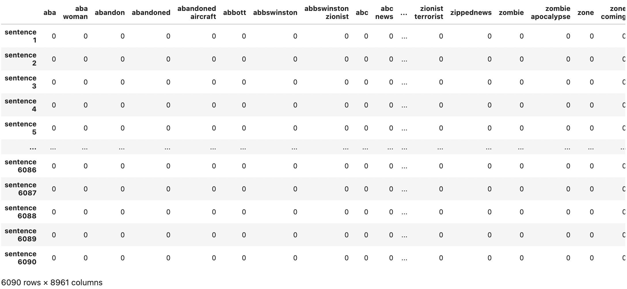
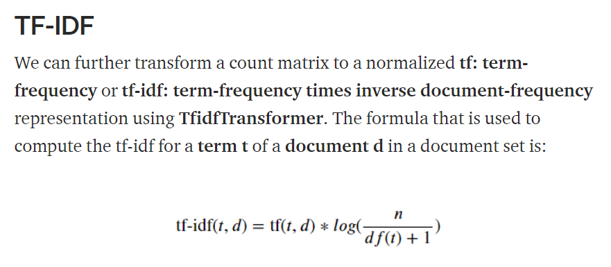

TfidfTransformer v.s. Tfidfvectorizer
두 개 모두 원시 상태의 텍스트 문서를 tf-idf 행렬로 만들어줍니다. 하지만 약간의 차이가 있습니다.
1. Tfidftransformer를 사용하려면 우리가 직접 Countvectorizer를 사용해 단어 등장 횟수를 체크하고, idf를 계산해야 합니다. 그 후에 tf-idf 점수만 계산해주게 됩니다.
2. 반면에 Tfidfvectorizer를 사용하면, 이 3가지 단계를 한 번에 수행할 수 있습니다.
# TfidfTransformer

from sklearn.feature_extraction.text import (CountVectorizer, TfidfVectorizer, TfidfTransformer)
vectorizer = CountVectorizer(analyzer='word', token_pattern=r'\b[a-zA-Z]{3,}\b', ngram_range=(1,1))
count_vectorized = vectorizer.fit_transform(x_train)
tfidf = TfidfTransformer(smooth_idf=True, use_idf=True)
train_features = tfidf.fit_transform(count_vectorized).toarray()

pd.DataFrame(train_features, index=['sentence '+str(i) for i in range(1, 1+len(x_train))], columns=vectorizer.get_feature_names_out())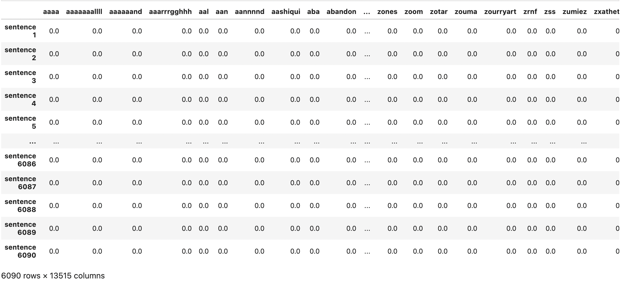
# TfidfVectorizer

# Convert a collection of text documents to a matrix of token counts

tfidf = feature_extraction.text.TfidfVectorizer(encoding='utf-8', ngram_range=(1,1), max_features=5000, norm='l2', sublinear_tf=True)
train_features = tfidf.fit_transform(x_train).toarray

pd.DataFrame(train_features, index=['sentence '+str(i) for i in range(1, 1+len(x_train))], columns=tfidf.get_feature_names_out())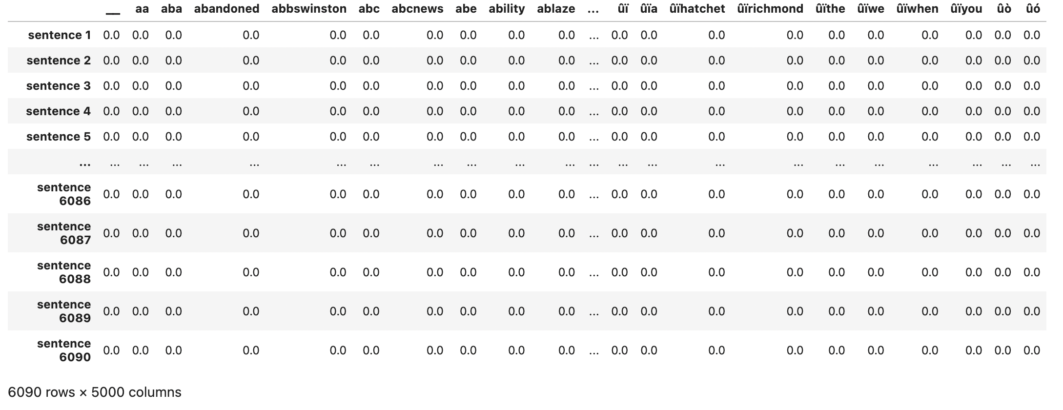
dic_vocabulary = tfidf.vocabulary_

word='forest'
dic_vocabulary[word]

# 만약 단어가 단어장에 있다면
# 출력으로 정수 N이 나옵니다.
# 이 정수가 의미하는 것은 행렬에서 이 단어가 몇 번째 피쳐인지입니다.

test_features = tfidf.transform(x_test).toarray()

train_labels = y_train
test_labels = y_test
모델 훈련
모델 : MultinomialNB
import pandas as pd
from sklearn.naive_bayes import MultinomialNB
from sklearn.metrics import classification_report, confusion_matrix, accuracy_score

mnb_classifier = MultinomialNB()
mnb_slcaasifier.fit(train_features, train_labels)

mnb_prediction = mnb_classifier.predict(test_features)
모델 성능 시각화
training_accuracy = accuracy_score(train_labels, mnb_classifier.preict(train_features))
print(training_accuracy)

#outputs
0.8691297208538588

testing_accuracy = accuracy_score(test_labels, mnb_prediction)
print(testing_accuracy)

#outputs
0.7905449770190414

print(classification_report(test_labels, mnb_prediction))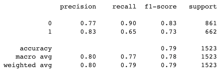
import seaborn as sns

conf_matrix = confusion_matrix(test_labels, mnb_prediction)

sns.heatmap(conf_matrix / np.sum(conf_matrix), annot=True, fmt='.2%', cmap='Blues')
제출 파일 만들기
test_vectorizer = tfidf.transform(data_clean_test['text_clean']).toarray()

final_predictions = mnb_classifier.predict(test_vectorizer)

submission_df = pd.DataFrame()
submission_df['id'] = data_clean_test['id']
submission_df['target'] = final_predictions
submission_df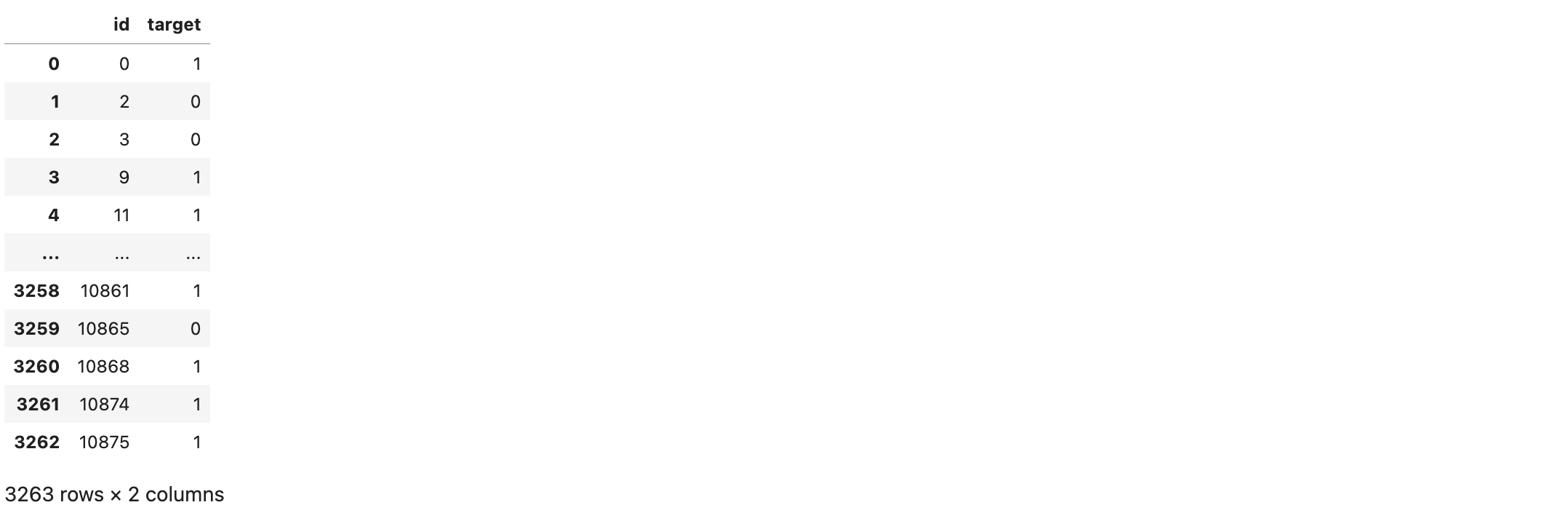
'Kaggle 필사 & 리뷰 > NLP' 카테고리의 다른 글
| [NLP] Kaggle 필사 커리큘럼(진행중) (0) | 2022.10.04 |
|---|---|
| Getting started with NLP - A general Intro (0) | 2022.09.12 |
| End-to-End NLP(EDA & ML) with Sentiment Analysis (0) | 2022.09.11 |

